Index
Overview
This document will describe how to export Statseeker’s API data to Grafana using the Grafana Infinity plugin. The Grafana Infinity plugin is a popular data source plugin that allows you to query and visualize data from various sources that don’t have native Grafana support, this includes Statseeker’s RESTful API.
Requirements
To follow this guide you will need the following:
- A Statseeker server (supported version)
- Statseeker user credentials for an account with API access
- Basic familiarity with the Statseeker API, its endpoints, and how to structure API requests
- A Grafana server (v10.4.8+) – https://grafana.com/grafana/download/
- Basic familiarity with Grafana, including how to create dashboards and panels
- Grafana Infinity Plugin installed on your Grafana server – https://grafana.com/grafana/plugins/yesoreyeram-infinity-datasource/
The Infinity plugin requires a Grafana version of 10.4.8 or later. In our example configuration we are using:
- Statseeker v25.3
- Grafana v12.3.1
- Grafana Infinity Plugin v3.7.0
- This document contains instructions and screenshot which are accurate for the product versions listed above, configuration details will vary for other versions of the Grafana Infinity plugin
- Both Grafana and the Infinity plugin are a third-party products and are not officially supported by Statseeker
Configuring the Statseeker Data Source
To configure Statseeker as a data source:
- Log in to your Grafana instance, typically this is at
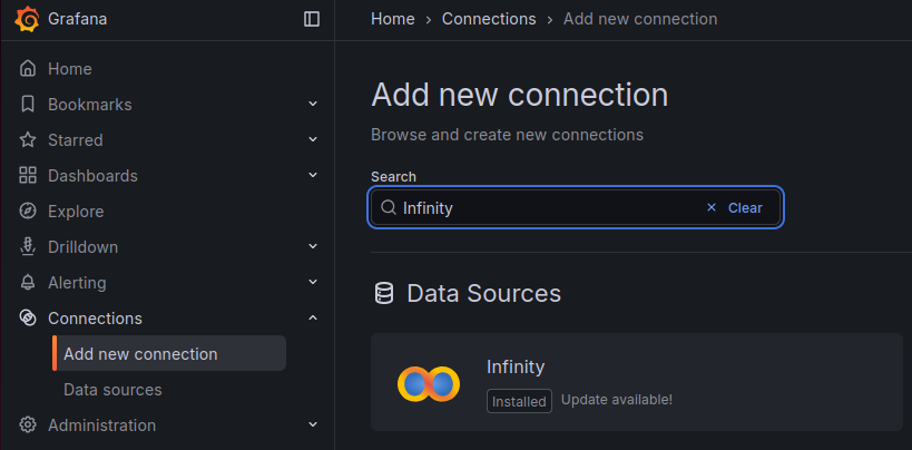
http://your-grafana-server:3000 - Select Connections > Add new Connection in the side menu (click the Grafana icon in the top-left if the sidebar is collapsed)
- Select the Infinity data source from the list and click Add new data source
- Configure:
- Click Save & Test
Authentication
Statseeker’s API supports Bearer Token (default) and Basic (deprecated) authentication methods. You will need to configure the authentication method in Infinity to match the method used by your Statseeker server. Both methods require credentials for a Statseeker user account with appropriate API and data permissions. For details on user account permissions, see Managing User Access & Permissions.

Basic Authentication
- Select Authentication and select Basic Authentication
- Enter the Username and Password for the selected Statseeker user account
Bearer Token Authentication
API tokens can be generated by sending a POST request to the Statseeker authentication endpoint (/ss-auth) with valid user credentials in the message body.
- Select Authentication and select Bearer Token
- Generate a valid API token (see below) in Statseeker (see API Tokens)
- Enter the Token for the selected Statseeker user account
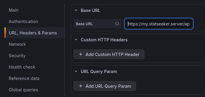
- Select URL, Headers & Params
- Set Base URL to your Statseeker API root endpoint (e.g.
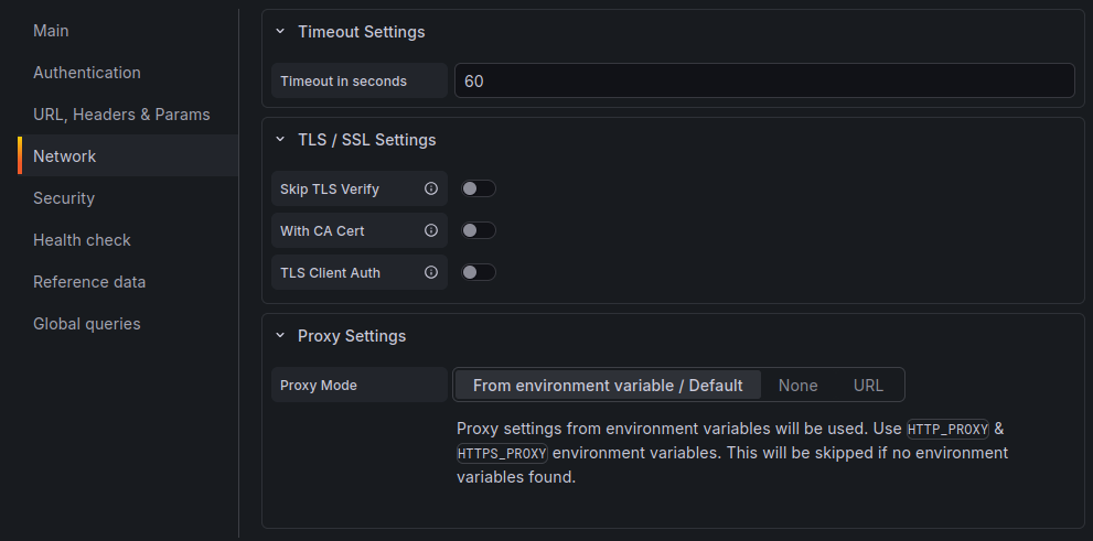
https://your.statseeker.server/api/latest) - Select Network
- Configure TLS/SSL Settings as needed for your environment
- Select Security
- Add your Statseeker server’s IP address or hostname to the Allowed Hosts list
- In Grafana, select Dashboards and then New
- Click Add visualization and select the configured Statseeker datasource if prompted
- Click Switch to table, setting the panel type to table, to view the response data
- Statseeker: fields=device,ipaddress,ping_state
- Grafana: fields=device&fields=ipaddress&fields=ping_state
- Visualization: Table
- URL: /cdt_device/?fields=name&fields=ping_state&fields=ipaddress&fields=ping_rtt&fields=ping_rtt_max&fields=ping_lost_percent&fields=ping_jitter&formats=avg&ping_lost_percent_formats=current&timefilter=range=now -10m to now&ping_state_filter=IS(“up”)
- Expand Parsing options & Result fields and set Rows/Root to data.objects[0].data, this will direct Grafana to look for rows of data at the specified location in the response
- Click on the Transform tab and click Add transformation
- Select Extract fields
- Set Source to the appropriate field name (e.g., ping_rtt, ping_rtt_max, etc.)
- Set Format to JSON
- Click Add path and set Field to the key within the JSON value (e.g., avg, max, etc.)
- Set Alias to a descriptive name for the column (e.g., “Average RTT”, “Max RTT”, etc.)
- Click Add another transformation and select Organize fields by name
- Use the eye icons to hide the original columns that contain the JSON values (e.g., ping_rtt, ping_rtt_max, etc.)
- Drag and drop the extracted metric columns to reorder them as needed
- Click on the column names to rename them as needed
- Click Back to dashboard to view the updated panel and Save the dashboard
- Visualization: Time Series
- URL: cdt_device/?fields=ping_rtt&formats=vals&formats=avg&value_time=start&fields=ping_state&ping_state_filter=IS(“up”)&fields=name&timefilter=range=now – 2h to now&groups=Routers&ping_rtt_sort=1&ping_rtt_sort=desc&ping_rtt_sort=avg&limit=5
- Expand Parsing options & Result fields and set Rows/Root to:
Statseeker authentication tokens are time-limited and will expire after a set period. If the bearer token specified in the datasource configuration expires, then communication between Grafana and Statseeker will fail until a new token is generated and updated in the datasource configuration. To avoid this, ensure that your Grafana dashboard refresh interval is set to a value that is shorter than the token’s time-to-live (TTL) so that the token will be automatically refreshed before it expires.
In the event that a previously working Grafana dashboard stops displaying Statseeker data, check that the Grafana server can still reach the Statseeker server. If it can, update the authentication token in the datasource configuration and refresh the dashboard.
URL, Headers & Params
Network
Security

Dashboards
Once the Connection/Datasource has been configured, you can create dashboards in Grafana that present Statseeker data. Each dashboard will consist or one or more panels, and panel configuration is going to vary with the specific data and visualization requirements of the panel, so we will work through a few examples.
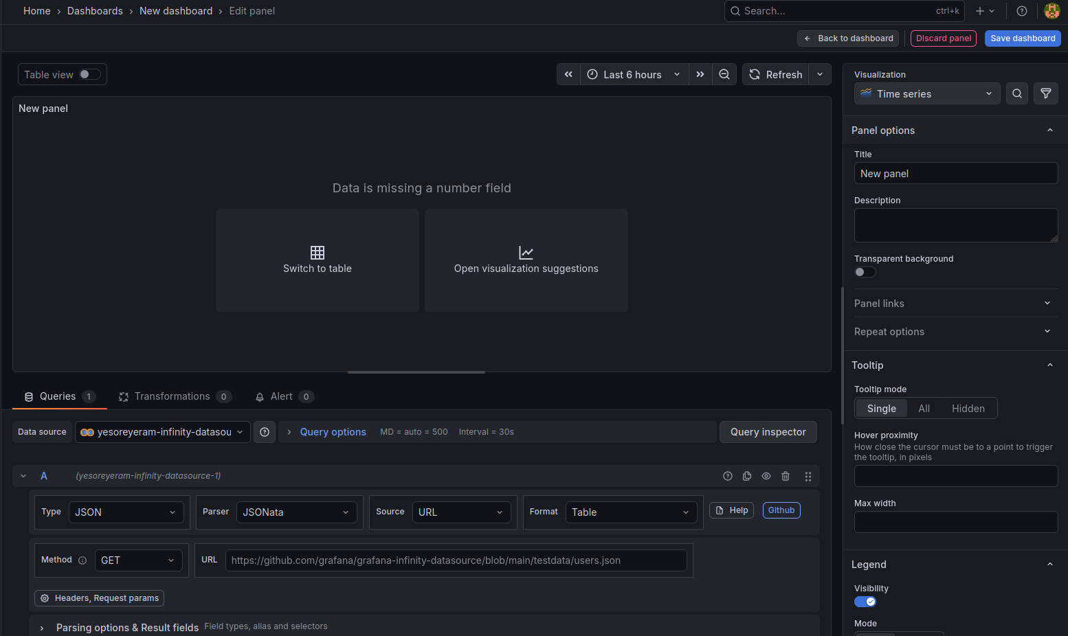
Grafana has already queried the Statseeker API referencing the the URL specified in the datasource configuration.
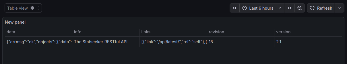
The base URl specified in the datasource configuration simply queries the API root endpoint, returning a list of the resource level endpoints available on your server. The URL field in the panel configuration can be used to modify the query being sent and return the data to be visualized in the panel.
We are going to query the cdt_device endpoint to return a range of ping data for each device.
The structure of query parameters provided to Grafana vary slightly from that used when querying the Statseeker API directly. Specifically, parameters that allow you to specify a list of comma-separated values must be repeatedly set for each value.
For example:
Lets look at a few panel configurations.
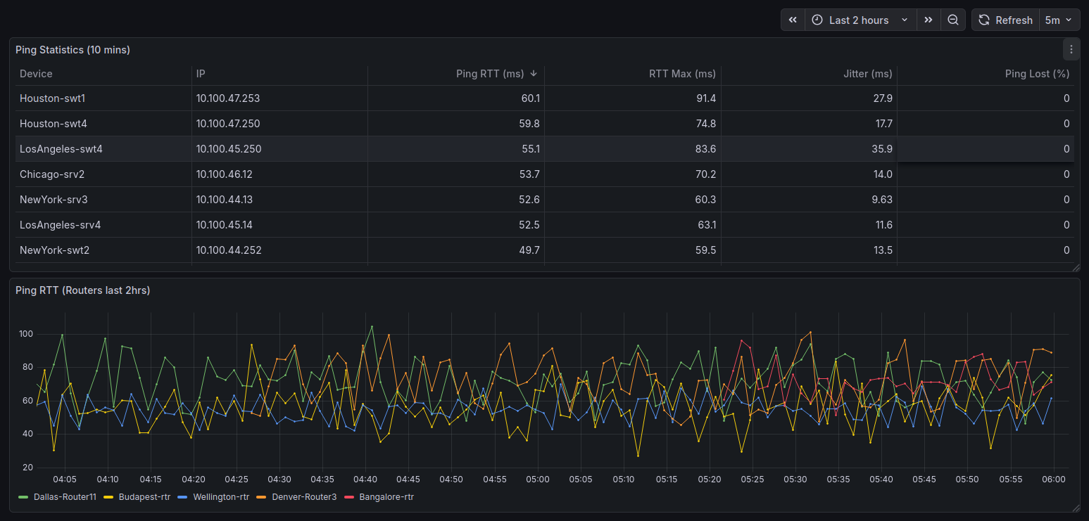
Ping Stats Table
In this example, we are creating a panel that displays ping statistics for each device in a table format. We will present the device name, IP address, current ping state, average round-trip time (RTT), maximum RTT, packet loss percentage, and jitter for the previous 10 minutes. We will also add a filter to only show devices that are currently “up”.
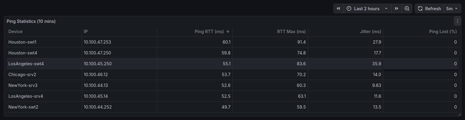

We can see that while device name and IP look ok, the time series metrics are being as a JSON key:value pair ({“avg”: 12.34}). We can format the the columns with data transformations.
For each of the timeseries metric columns:
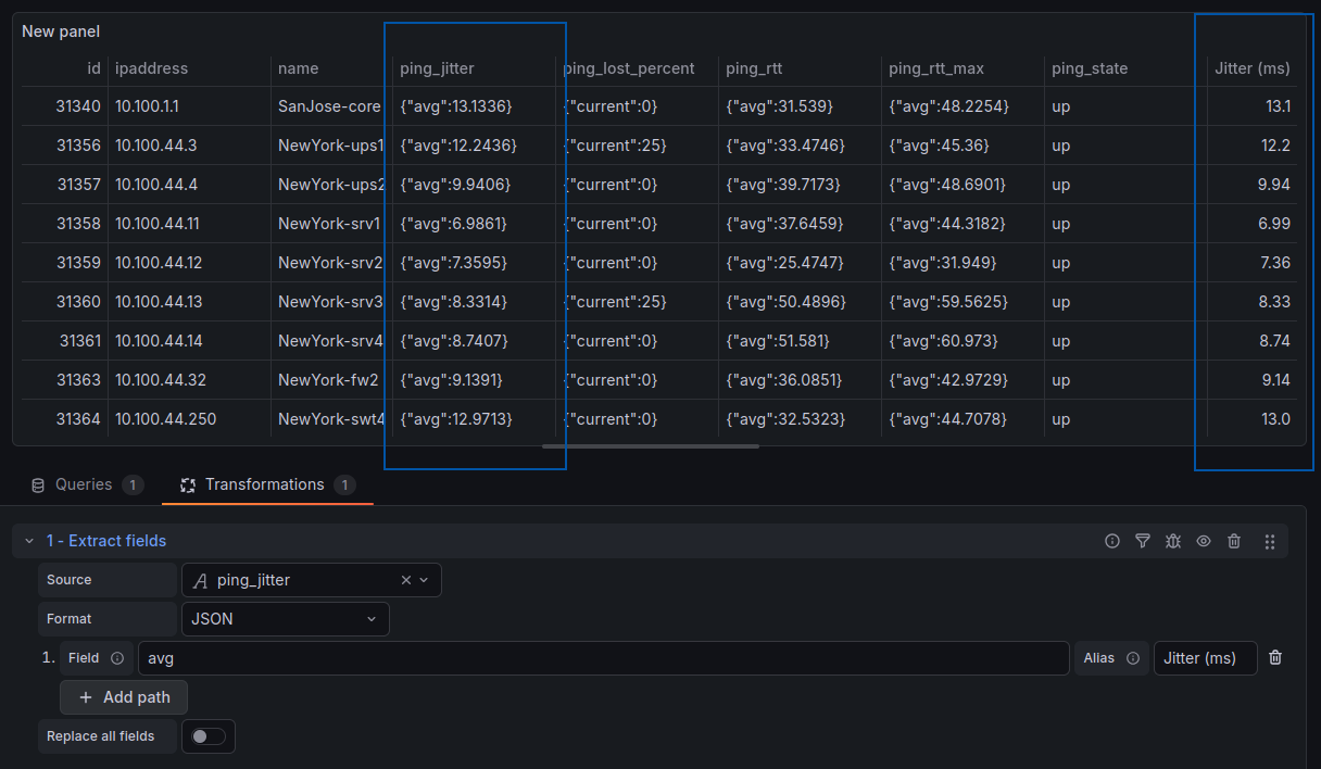
We can use another transformation to hide the duplicate columns as well as rename and reorder them as needed.

Ping RTT Graph
In this example, we are creating a panel that graphs ping RTT over the last 2 hours. This data is filtered to devices in my Routers groups and limited to the 5 devices with the highest average ping RTT over that period. We will be using the default JSONata back-end parser, an alternate configuration is also provided using the UQL front-end parser.
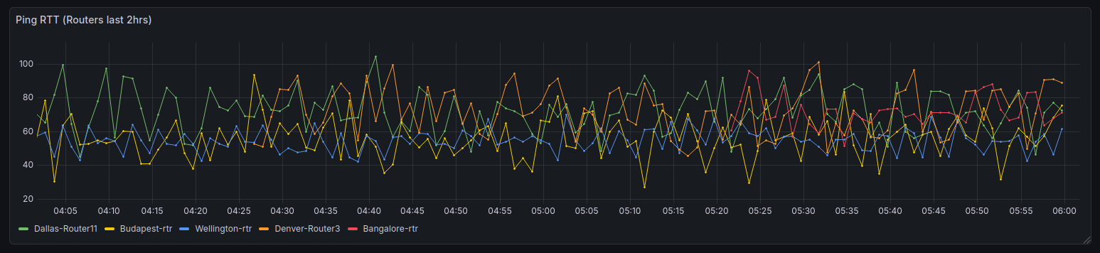
To plot data over time, Grafana requires that we return timestamps for each data point, so we have to include a value_time parameter.
When formats=vals, Statseeker returns the data as nested arrays so we need a little more configuration than we saw in the previous table configuration.
data.objects[0].data.(
  $device := name;
  ping_rtt.vals[$type($[0]) = "number" and $type($[1]) = "number"].{
    "time": $number($[0]) * 1000,
    "value": $number($[1]),
    "device": $device
  }
)
This instructs Grafana to look for data points in the ping_rtt.vals field, extract the timestamp and value from the nested arrays, and also include the device name as a label for each data point. We also need to instruct Grafana on how to interpret the data.
- In Parsing options & Result fields, click Add column
- Select Selector to the current column header
- Set Title to the display label for the value
- Set format as to the required data-type
- device : Device : String
- time : Time : Time (Unix ms)
- value : Ping RTT : Number

If we hit Refresh, we can see data in the graph, but everything is rendered as a single series. We add a Transformation to separate the series.
- Click Transformations, then Add transformation
- Select Prepare time series and set Format = Multi-frame time series
![]()
- Set the dashboard timefilter to match the original query’s time range and click Apply time range

By default, the graph legend displays the series names as the conjunction of the 2 non-value column headers. There are a couple ways to address this, either:
- In Parsing options & Result fields set the value column’s title to a single space
- Or, in the Visualization configuration (right-panel), set Display name to ${__field.labels.Device}
- Click Refresh
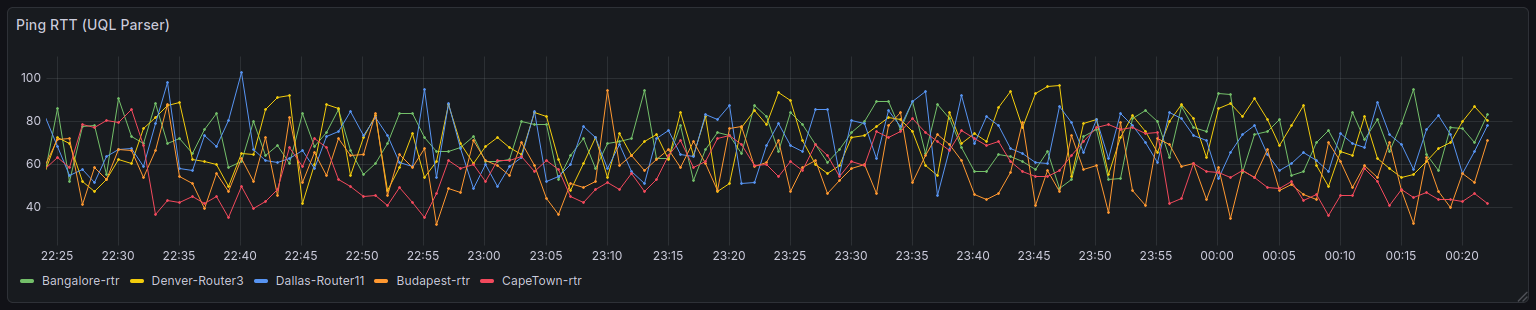
Ping RTT Graph (UQL front-end parser)
As an alternative to the JSONata back-end parser, we can use the UQL front-end parser to simplify the configuration when dealing with nested data. In this example we reproduce the same result as in the previous example, using the UQL parser.
- Visualization: Time Series
- Parser: UQL
- URL: cdt_device/?fields=ping_rtt&formats=vals&formats=avg&value_time=start&fields=ping_state&ping_state_filter=IS(“up”)&fields=name&timefilter=range=now – 2h to now&groups=Routers&ping_rtt_sort=1&ping_rtt_sort=desc&ping_rtt_sort=avg&limit=5 – the same query as the previous example
- Expand the UQL section and set the UQL Query to:
parse-json
| scope "data.objects[0].data"
| mv-expand "ping"="ping_rtt.vals"
| project "Device"="name", "Time"=unixtime_seconds_todatetime("ping.[0]"), "Value"=tonumber("ping.[1]")
- Click Transformations, then Add transformation
- Select Prepare time series and set Format = Multi-frame time series
- Set the dashboard timefilter to match the original query’s time range and click Apply time range